
When working with brain data, one of the biggest challenges is making sense of complex patterns hidden in signals like EEG. Each second of brain activity produces thousands of data points that reflect subtle changes in cognitive and emotional states. Visualizing this high-dimensional information can help us uncover meaningful relationships that numbers alone can’t show. In this post, we use UMAP, a modern dimensionality-reduction technique, to explore whether we can find structure in EEG Power Spectral Density (PSD) data, essentially, the “frequency fingerprint” of the brain. Our goal is to see if meaningful patterns emerge that relate to brain states, tasks, or individuals.
Although this topic sits at the intersection of neuroscience and data science, we’ve written it in a way that’s accessible beyond research labs. The main audience is data scientists, but we’ve kept explanations intuitive and added a few business-relevant analogies along the way.
Context & Motivation
EEG data, like many biological signals, are inherently high-dimensional. Each channel, frequency band, and time window adds another layer of complexity. To visualize or interpret such data, we often need to reduce its dimensionality, compressing hundreds of features into two or three dimensions while preserving the relationships between samples. Traditional methods like Principal Component Analysis (PCA) capture global variance but may miss non-linear relationships. More recent approaches like t-SNE and UMAP go further, preserving local structure and neighborhood relationships in complex datasets. In this analysis, we use UMAP because it balances global and local preservation, scales efficiently to large datasets, and produces visualizations that reveal meaningful manifolds rather than isolated clusters. It helps us see how EEG power spectra are organized, whether by brain state, region, or individual differences.
By using UMAP, we uncover a layered hierarchy within EEG Power Spectral Density (PSD) data, where physiological states (such as eyes open vs. closed) and individual differences dominate over task-related variations. In other words, the brain’s spectral patterns are first shaped by state, then by anatomical region, then by subject-specific traits, and only subtly by task. This hierarchy suggests that uncovering task-related brain states is inherently more challenging and requires careful modeling to separate these overlapping influences.
Dataset
The dataset comprises 12,888 samples, each representing a 40-dimensional Power Spectral Density (PSD) vector corresponding to frequencies from 1 Hz to 40 Hz, derived from a 1-minute EEG segment recorded from a single channel. Data were collected across three experiments: Stroop, Arithmetic Operation, and Watching Driving Videos. The Stroop task is a well-known cognitive interference task that measures attention and cognitive control by asking participants to name the color of a word that may conflict with its semantic meaning (e.g., the word “red” written in blue ink). The Arithmetic Operation task involved solving mental calculations designed to increase cognitive load; therefore, we refer to it as MW (Mental Workload) in the following. The same 19-channel EEG device was used consistently in all experiments, with A1 as the reference electrode, and all signals were resampled to 128 Hz.
Each experimental session includes a task segment, which may have multiple phases, along with pre- and post-task rest data, with Eye Open (EO) and Eye Closed (EC) segments. There are 29 subjects in total, with each subject participating in one, two, or all three experiments.
The total labeled data amounts to 690 minutes, recorded across 19 channels. This initially yielded 13,110 channel-window samples, which were subsequently refined to 12,888 after cleaning and removing poor-quality data. For PSD computation, only clean segments of the EEG were used. To find the clean segments of the EEG, we used the InnoBrain cleaning algorithm. A window is dropped exclusively when it contains insufficient clean data.
The UMAP algorithm was applied to the data using a Euclidean metric, with the number of dimensions set to 2, the number of neighbors set to 30, and the minimum distance set to 0.1.
Result
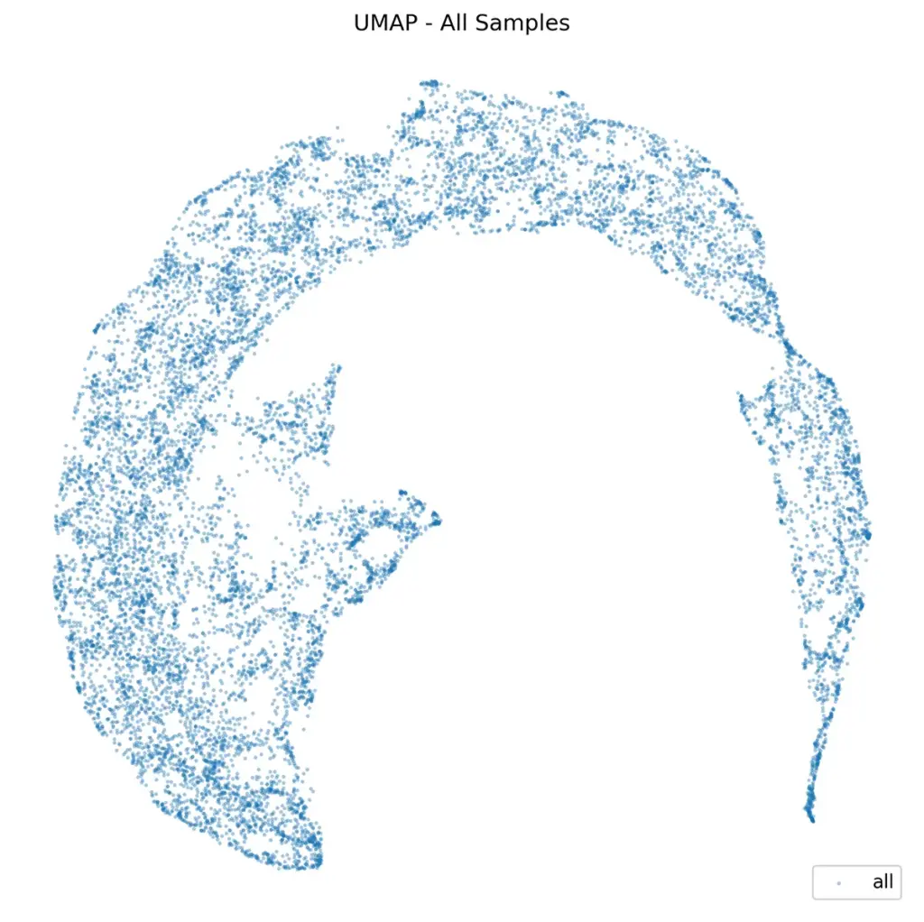 Figure 1. 2-d UMAP of all samples.
Figure 1 illustrates the UMAP, which presents as an almost continuous spread rather than showing distinct clusters, even after various parameter adjustments. Only two minor groups appear near the center, suggesting that PSD varies gradually and continuously rather than forming discrete, well-separated categories.
Next, we will apply different coloring schemes, that is, we will color the data points in the UMAP plot according to various variables such as brain region, eye-open/eye-closed state, subject ID, or experiment type. This allows us to visually examine whether the observed clusters correspond to any of these factors. Before proceeding, consider what you anticipate observing: Do you expect distinct groupings by brain region, or separations based on the eye-open and eye-closed states? Do you expect clustering by subjects or by experimental conditions?
Eye Open (EO) vs. Eye Closed (EC)
The first comparison we looked at was between eye-open and eye-closed states. Considering only rest data, distinguishing between EO and EC is very easy in both time and power domains, as EC has a high level of alpha oscillations. So we expect to see different segments for them in UMAP. Figure 2 shows this coloring.
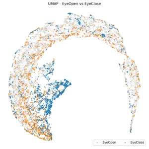
Figure 2. UMAP of Rest data. EC and EO are in different clusters.
In the UMAP space, two small clusters in the center are associated with EC, while the remaining area is filled by EO. EO and EC are distinct within the UMAP space. A K-nearest neighbors (KNN) classification with K=10, using their UMAP embedding, yields a balanced accuracy of 74% using 5-fold cross-validation, indicating that the embedding effectively preserves meaningful distinctions between the two eye states and captures physiologically relevant structure in the data.
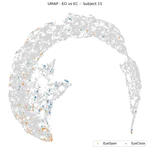
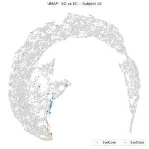
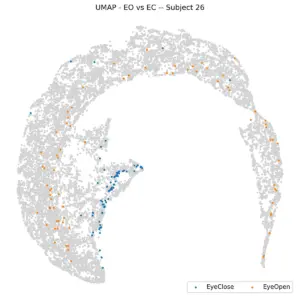
Examining individual subjects, the plot below shows the same visualization for six randomly selected participants. Most subjects display a consistent pattern, with eyes-closed (EC) data clustered near the center and eyes-open (EO) data distributed toward the periphery. However, this pattern is not universal, as illustrated by Subject 1. Overall, while each subject tends to exhibit a similar relative organization of EO and EC data, the absolute positioning of clusters varies across individuals. This variability suggests that although the within-subject structure is stable, the embedding does not generalize well across subjects, making it difficult to determine the eye state of a new subject solely based on spatial location in the UMAP space.
 |
 |
 |
 |
 |
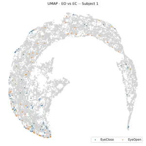 |
Figure 3. UMAP of Rest data per individual subjects. EC and EO are in different clusters.
Brain Regions
While it’s very easy for EEG experts to differentiate various brain regions in the time domain due to the influence of eye-blink artifacts and their distinct effects on different areas, this task becomes challenging even for experts if the noise is removed and the data is viewed in the Power Spectral Density (PSD) domain as we anticipate a higher alpha presence in the posterior region and a lower alpha presence in the anterior region.
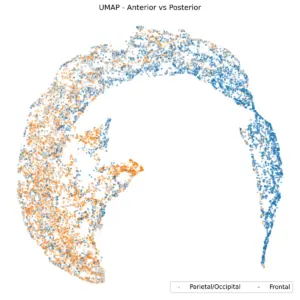
Figure 4. UMAP, based on the brain region.
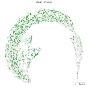
Figure 4 shows UMAP based on the brain region. Frontal channels are distinctly separate from parietal and occipital channels. A K-nearest neighbors (KNN) classification with K=10, using anterior/posterior UMAP embedding, yields a balanced accuracy of 80%. Central and temporal channels, as shown in the subsequent two plots, are positioned between the anterior and posterior regions.
 |
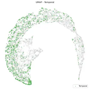 |
Figure 5. UMAP of Central and Temporal regions.
An interesting question arose regarding the frontal EC samples: Would they align with the EC region or the frontal region? The following figure demonstrates that the EC region exerts a stronger influence, leading these samples to be part of the EC cluster.
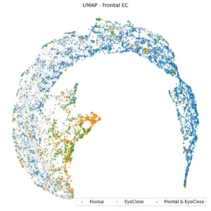
Figure 6. UMAP embedding of frontal EC is a part of the EC region.
Tasks and Subjects
We then turned to the question of task separability. We are investigating three distinct tasks: Stroop, MW, and Driving. These tasks are quite different, and we anticipate that their respective EEGs will allow for their prediction. However, relying solely on the Power Spectral Density (PSD) of a single channel over one minute might be an overly optimistic expectation. This can also be examined by the UMAP. To eliminate subject variability, we focused on the Stroop and MW tasks. This decision was based on the fact that six subjects participated in both experiments, allowing us to plot data exclusively from these individuals.
 |
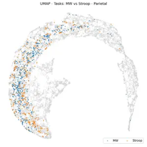 |
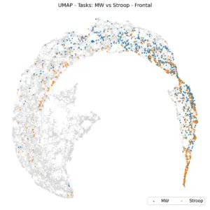
Figure 7. UMAP projections based on tasks. Left: Frontal, Right: Parietal.
Figure 7 illustrates UMAP coloring according to tasks within frontal (left) and parietal (right) regions for 6 shared subjects. The K-Nearest Neighbors (KNN) balanced accuracy is 61% for frontal and 62% for parietal, which is an improvement over random chance, indicating that task effects are subtle at this level of representation. This raises the question: if we analyze task predictability per subject, do tasks become more distinctly separated?
 |
 |
 |
 |
 |
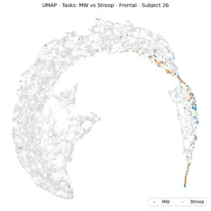 |
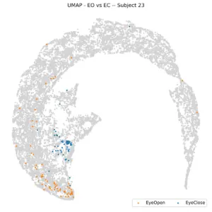
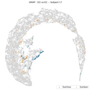
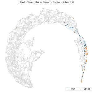
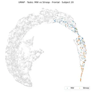
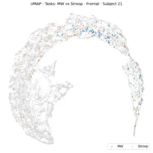
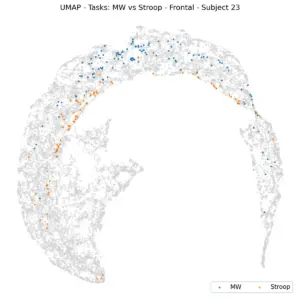
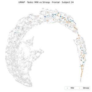
Figure 8. UMAP of tasks per individual subjects.
Figure 8 illustrates this concept for individual subjects, revealing a non-uniform distribution within the frontal regions. For instance, subject 23 is situated in the left frontal region, while subject 17 is on the right. However, separating the dataset by subject appears to simplify analysis, a finding supported by KNN. When subject-specific KNN is applied and the average of balanced accuracies is calculated, the result is 73%, a significant improvement over 61%. This leads us to fix the task (e.g., to Stroop) and color the UMAP by subjects to check subject separability.
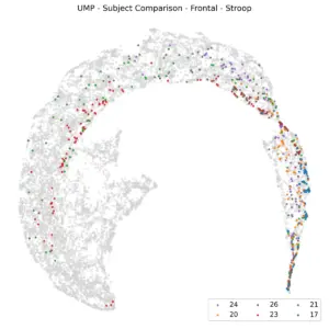
Figure 9. UMAP of frontal Stroop per subject.
Figure 9 displays the frontal channels of the Stroop task for selected subjects, revealing distinct subject clusters. The K-Nearest Neighbors (KNN) model achieved a balanced accuracy of 49%, a significant improvement over the 16.6% random accuracy. This indicates that subjects are not uniformly distributed and tend to form their own clusters, which could lead to reduced task accuracy, particularly when considering subject-independent accuracies.
Conclusion
Taken together, these results reveal a hierarchy in EEG PSD structure. The strongest separability comes from physiological state, with the eye closed and the eye open forming distinct patterns. Brain regions are next, with anterior and posterior channels separating clearly. Subjects then form their own identifiable clusters, and only after these factors do task differences begin to emerge. This hierarchy suggests that state and subject factors can easily mask task-related effects unless they are carefully controlled or normalized.
UMAP proves to be a powerful tool for exploring these relationships. It shows that EEG data is not neatly divided into discrete clusters but instead lies on a continuous manifold, shaped most strongly by state, then by anatomical region, then by individual traits, and finally by task.